Advanced Simulator Features
Note:
All following examples are important features of the ctRSD-simulator-2.0.
Note the code blocks illustrate how to set examples up for a single set of initial conditions. The Python scripts on GitHub work through testing many different initial conditions, i.e., changing which inputs are present.
Discontinuous Simulation
Discontinuous Simulation provides guidance for the usage of discontinuous feature of ctRSD-simulator-2.0. This feature allows the user to run a simulation for a specific amount of time using any desired conditions, and then apply a different set of conditions for the next time span, until the end of the simulation. The user has the ability to change the conditions for a given amount of time across the entire length of the simulation as many times as needed. Also, full function of the different features of the simulator are available to be changed for different time spans of the total simulaton time. In the example script, G{1,2} is transcribed alongside a R{2} for 60 min and then the template for I{1} is added.
Note:
The discontinuous feature is a part of the simulate function. More information on using simulate for discontinuous simulations can be found here
- Useful Features:
discontinuous simulation feature in simulate()
globally changing rate constants with global_rate_constants()
changing indiviudal rate constants within molecular_species
Discontinuous Simulation Python Script can be found here
# auxiliary packages needed in the script below, e.g., plotting
import numpy as np
import matplotlib.pyplot as plt

# importing simulator
import sys
sys.path.insert(1,'filepath to simulator location on local computer')
import ctRSD_simulator_200 as RSDs # import latest version of the simulator


# create the model instance
model = RSDs.RSD_sim() # default # of domains (5 domains)

# specify species involved in the system
model.molecular_species('G{1,2}',DNA_con=25)
model.molecular_species('R{2}',ic=500)

# simulating the model for 1 hour
t_sim = np.linspace(0,1,1001)*3600 # seconds
model.simulate(t_sim) # simulate the model

# adding the I{1} template to the model
model.molecular_species('I{1}',DNA_con=25)

# continue simulation with I{1} template added for 3 more hours
t_sim2 = np.linspace(t_sim[-1]/3600,4,1001)*3600 # seconds
model.simulate(t_sim2,iteration=2) #must specify it is second iteration

# pulling out the reporter concentration for plotting
S2 = model.output_concentration('S{2}')

# simple plotting code
plt.plot(t_sim,S2,color='blue')
plt.xlabel('Time (s)')
plt.ylabel('Concentration (nM)')
Discontinuous Simulation
Degradation Simulation
Degradation Simulation shows the ability to use global_rate_constants to raise degradation rates from their 0 default to initialize degradation reactions in a system.
global_rate_constants() gives the user the ability to change all degradation rates at once using “kdeg” as an argument, to just change degradation rates for single stranded species,”kssd,” double stranded species,”kdsd,” or RNA:DNA hyrbids,”kdrd,” and finally to change the degrdation rates for any given individual species.
The following two figures change all degradation rates simultaneously.
- Useful Features:
incorporating degradation reactions
globally changing rate constants with global_rate_constants()
changing indiviudal rate constants within molecular_species()
Degredation Simulation Python Script can be found here
# auxiliary packages needed in the script below, e.g., plotting
import numpy as np
import matplotlib.pyplot as plt

# importing simulator
import sys
sys.path.insert(1,'filepath to simulator location on local computer')
import ctRSD_simulator_200 as RSDs # import latest version of the simulator


# create the model instance
model = RSDs.RSD_sim() # default # of domains (5 domains)

#globally changes all degradation rates
model.global_rate_constants(kdeg=0.001)

# specify species involved in the system
model.molecular_species('I{1}',DNA_con=25)
model.molecular_species('G{1,2}',DNA_con=25)
model.molecular_species('R{2}',ic=500)

# simulating the model
t_sim = np.linspace(0,3,1001)*3600 # seconds
model.simulate(t_sim) # simulate the model

# pull out the species from the model solution to plot
S2 = model.output_concentration('S{2}')

# simple plotting code
plt.plot(t_sim,S2,color='blue')
plt.xlabel('Time (s)')
plt.ylabel('Concentration (nM)')
Degradation Simulation
The following degredation example simulates a system with degradation rates where single stranded species, double stranded species, and RNA in RNA:DNA hyrbids are all independently changed.
Degradation Simulation with changing groups of rates Python Script can be found here
# auxiliary packages needed in the script below, e.g., plotting
import numpy as np
import matplotlib.pyplot as plt

# importing simulator
import sys
sys.path.insert(1,'filepath to simulator location on local computer')
import ctRSD_simulator_200 as RSDs # import latest version of the simulator


# create the model instance
model = RSDs.RSD_sim() # default # of domains (5 domains)

# globally changes specific types of degradation rates (below are some example commands)
model.global_rate_constants(kssd=0.001) # to change only ssRNA degradation rates
# model.global_rate_constants(kdsd=0.001) # to change only dsRNA degradation rates
# model.global_rate_constants(kdrd=0.001) # to change only RNA in RNA:DNA complex degradation rates
# model.global_rate_constants(kssd=0.001,kdsd=0.001,kdrd=0.001) # to change all three above together

# specify species involved in the system
model.molecular_species('I{1}',DNA_con=25)
model.molecular_species('G{1,2}',DNA_con=25)
model.molecular_species('R{2}',ic=500)

# simulating the model
t_sim = np.linspace(0,3,1001)*3600 # seconds
model.simulate(t_sim) # simulate the model

# pull out the species from the model solution to plot
S2 = model.output_concentration('S{2}')
I1 = model.output_concentration('I{1}')
G12 = model.output_concentration('G{1,2}')
O12 = model.output_concentration('O{1,2}')

# simple plotting code
plt.subplot(2,4,1)
plt.plot(t_sim,I1,color='blue')
plt.xlabel('Time (s)')
plt.ylabel('Concentration (nM)')

plt.subplot(2,4,2)
plt.plot(t_sim,G12,color='blue')
plt.xlabel('Time (s)')
plt.ylabel('Concentration (nM)')

plt.subplot(2,4,3)
plt.plot(t_sim,O12,color='blue')
plt.xlabel('Time (s)')
plt.ylabel('Concentration (nM)')

plt.subplot(2,4,4)
plt.plot(t_sim,S2,color='blue')
plt.xlabel('Time (s)')
plt.ylabel('Concentration (nM)')
Degradation Simulation (Changing Groups of Degradation Rates)
Two-Toehold Cascade Simulation
This simulation demonstrates a 4-layer cascade in which gates of every other layer have different strand displacement rate constants. This mimics a system with two input-output toeholds that alternate between layers and have different rate constants.
- Useful Features:
using expanded experimental nomenclature when specifying components within molecular_species()
globally changing rate constants with global_rate_constants()
changing indiviudal rate constants within molecular_species()
Two-Toehold Simulation
Two Toehold Sim Python Script can be found here
'''
This example shows just the 4-layer cascade
'''

# auxiliary packages needed in the script below, e.g., plotting
import numpy as np
import matplotlib.pyplot as plt

# importing simulator
import sys
sys.path.insert(1,'filepath to simulator location on local computer')
import ctRSD_simulator_200 as RSDs # import latest version of the simulator


# create the model instance
model = RSDs.RSD_sim() # default # of domains (5 domains)

#globally changing transcription rate constant
model.global_rate_constants(ktxn=0.0075)

# specify species involved in the system
model.molecular_species('I{u3}',DNA_con=25)

kvth=5e3/1e9 # specifying a faster rate constant for v toeholds
model.molecular_species('G{u3,v4}',DNA_con=25)
model.molecular_species('G{v4,u5}',DNA_con=25,krsd=kvth)
model.molecular_species('G{u5,v1}',DNA_con=25)
model.molecular_species('G{v1,u2r}',DNA_con=25,krsd=kvth)

model.molecular_species('R{u2}',ic=500)

# simulating the model
t_sim = np.linspace(0,3,1001)*3600 # seconds
model.simulate(t_sim) # simulate the model

# pull out the species from the model solution to plot
S2 = model.output_concentration('S{2}')

# simple plotting code
plt.plot(t_sim,S2,color='blue')
plt.xlabel('Time (s)')
plt.ylabel('Concentration (nM)')
AND Gate with Fuel Simulation
This simulation shows a basic ctRSD AND gate system, but with fuel added to one of the inputs using molecular_species
- Useful Features:
specifying AND gates in molecular_species()
specifying fuel strands in molecular_species()
changing indiviudal rate constants within molecular_species()
changing initial conditions within molecular_species()
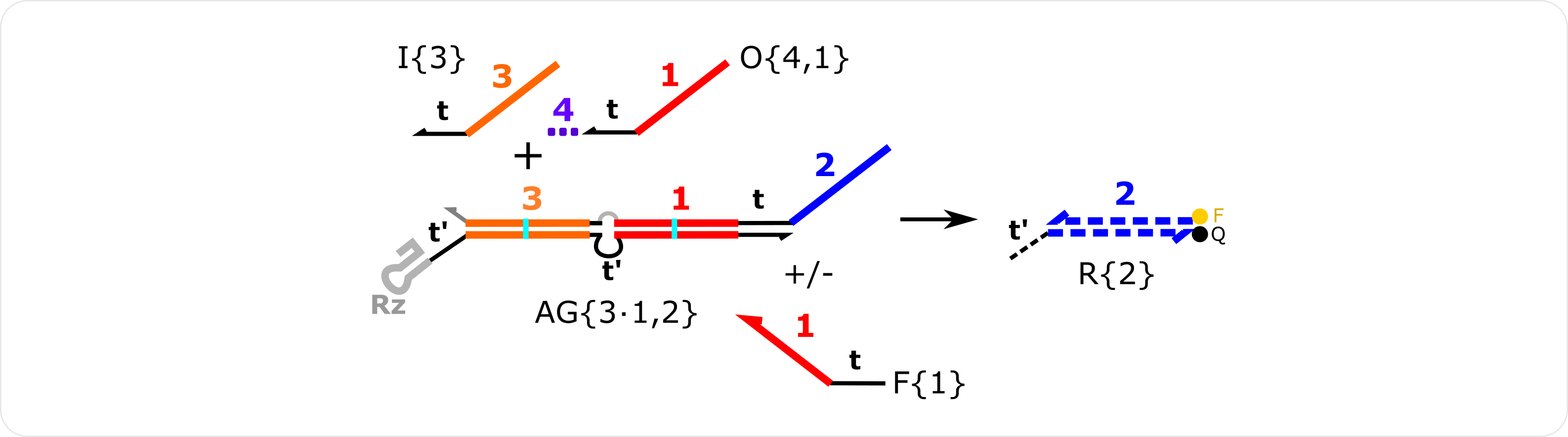
AG Fuel Simulation
AG Fuel Sim Python Script can be found here
# auxiliary packages needed in the script below, e.g., plotting
import numpy as np
import matplotlib.pyplot as plt

# importing simulator
import sys
sys.path.insert(1,'filepath to simulator location on local computer')
import ctRSD_simulator_200 as RSDs # import latest version of the simulator


# create the model instance
model = RSDs.RSD_sim() # default # of domains (5 domains)

# specify species involved in the system
model.molecular_species('I{3}',DNA_con=25)
model.molecular_species('O{4,1}',DNA_con=1.25) # limiting second input to the AG

model.molecular_species('AG{3.1,2}',DNA_con=25)
model.molecular_species('R{2}',ic=500)

model.molecular_species('F{1}',DNA_con=25)

# simulating the model
t_sim = np.linspace(0,3,1001)*3600 # seconds
model.simulate(t_sim) # simulate the model

# pull out the species from the model solution to plot
S2 = model.output_concentration('S{2}')

# simple plotting code
plt.plot(t_sim,S2,color='blue')
plt.xlabel('Time (s)')
plt.ylabel('Concentration (nM)')
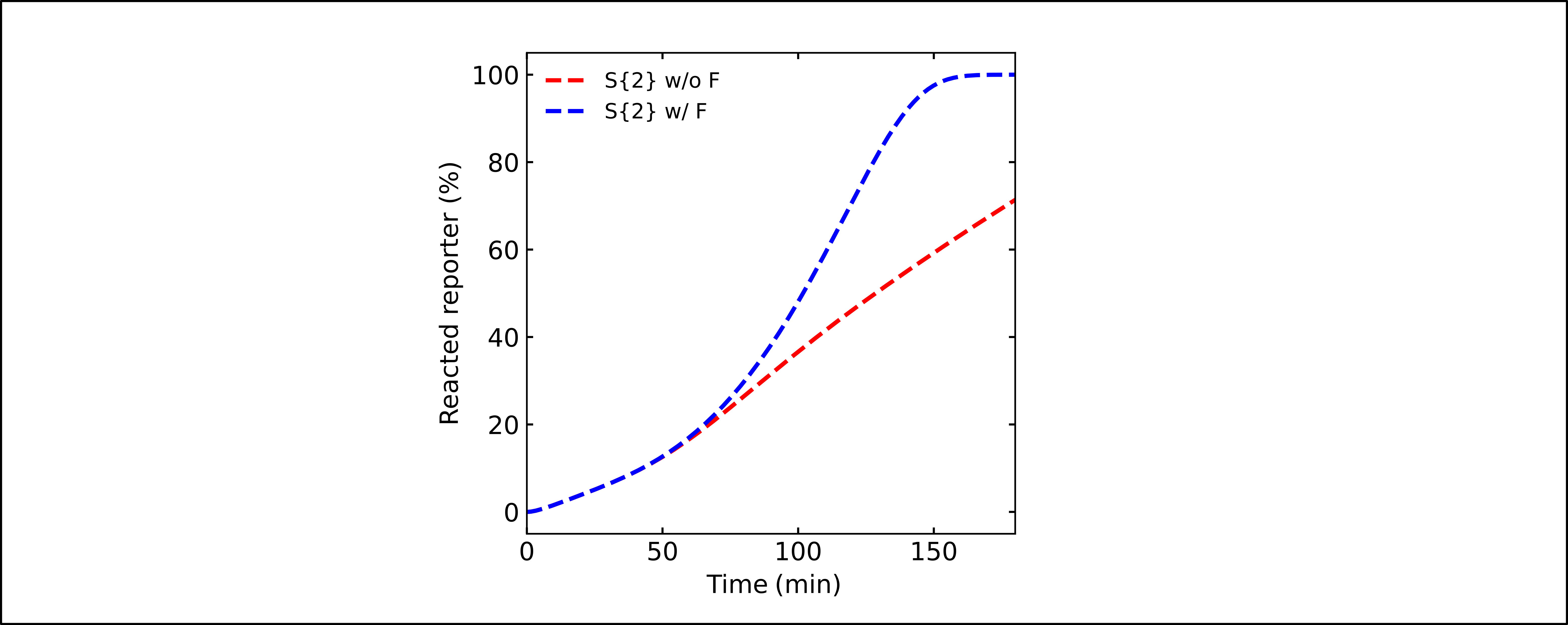
AG + Fuel Simulation Results
Two AND Gate OR Simulation
This simulation shows a 4-input circuit composed of 2 ctRSD AND gates that both produce the same output ( ex. (A AND B) OR (C AND D) ).
- Useful Features:
specifying AND gates in molecular_species()
changing indiviudal rate constants within molecular_species()
changing initial conditions within molecular_species()
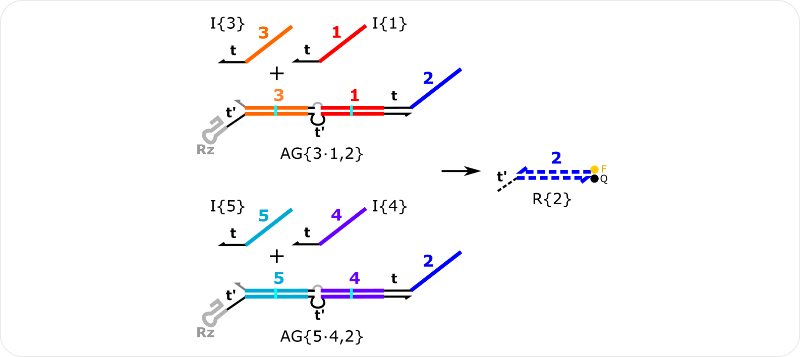
Two AND Gate OR Simulation
Two AND gate OR Simulation Python Script can be found here
# auxiliary packages needed in the script below, e.g., plotting
import numpy as np
import matplotlib.pyplot as plt

# importing simulator
import sys
sys.path.insert(1,'filepath to simulator location on local computer')
import ctRSD_simulator_200 as RSDs # import latest version of the simulator


# create the model instance
model = RSDs.RSD_sim() # default # of domains (5 domains)

# specify species involved in the system
model.molecular_species('I{1}',DNA_con=0)
model.molecular_species('I{3}',DNA_con=0)
model.molecular_species('I{4}',DNA_con=25)
model.molecular_species('I{5}',DNA_con=25)

model.molecular_species('AG{5.4,2}',DNA_con=25)
model.molecular_species('AG{3.1,2}',DNA_con=25)
model.molecular_species('R{2}',ic=500)

# simulating the model
t_sim = np.linspace(0,3,1001)*3600 # seconds
model.simulate(t_sim) # simulate the model

# pull out the species from the model solution to plot
S2 = model.output_concentration('S{2}')

# simple plotting code
plt.plot(t_sim,S2,color='blue')
plt.xlabel('Time (s)')
plt.ylabel('Concentration (nM)')
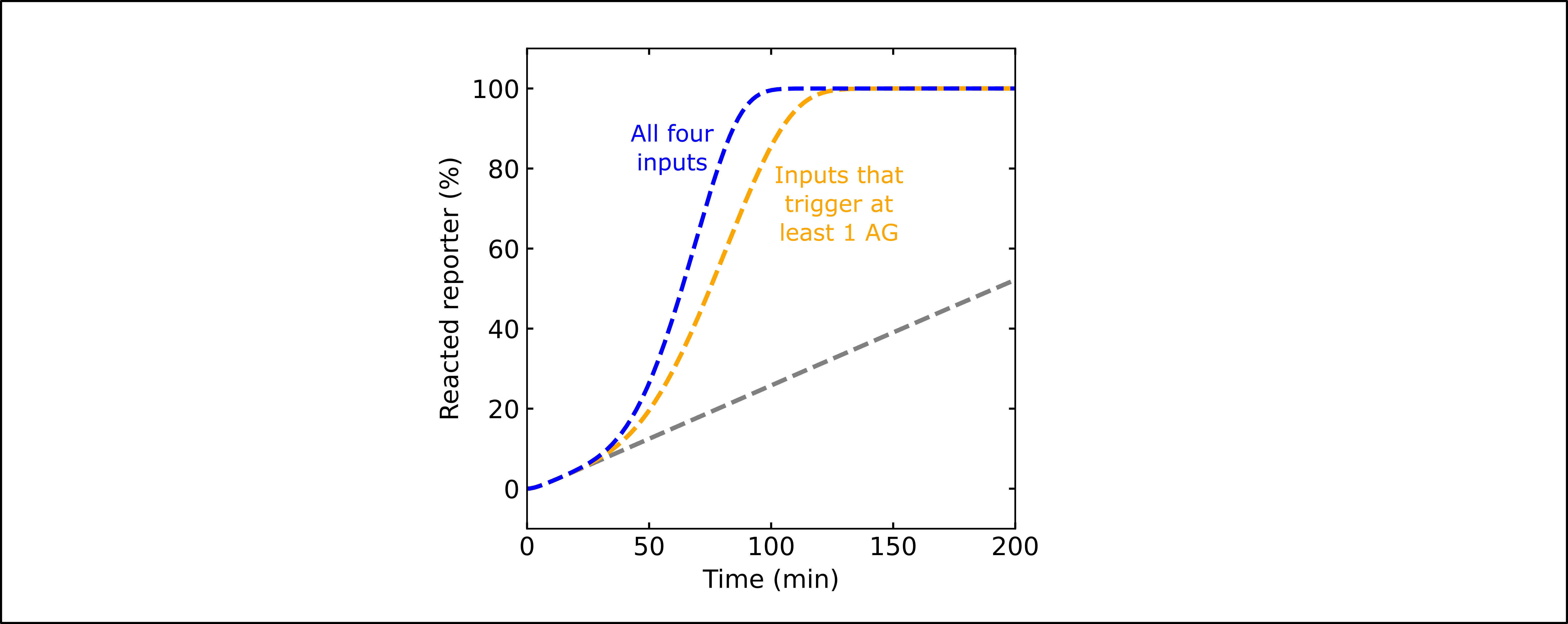
Two AND Gate OR Simulation Results
Thresholding Simulation
Thresholding Simulation showcases a simple thresholding reaction, where a threshold gate is produced to effectively annihlate input produced at a rate below the threshold gate.
- Useful Features:
specifying threshold gates in molecular_species()
globally changing rate constants with global_rate_constants()
changing indiviudal rate constants within molecular_species()
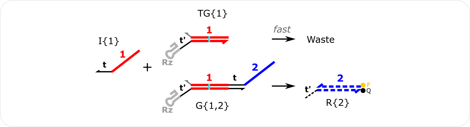
Thresholding Simulation
Thresholding Simulation Python Script can be found here
# auxiliary packages needed in the script below, e.g., plotting
import numpy as np
import matplotlib.pyplot as plt

# importing simulator
import sys
sys.path.insert(1,'filepath to simulator location on local computer')
import ctRSD_simulator_200 as RSDs # import latest version of the simulator


# create the model instance
model = RSDs.RSD_sim() # default # of domains (5 domains)

# specify species involved in the system
model.molecular_species('I{1}',DNA_con=25)

model.molecular_species('G{1,2}',DNA_con=25)
model.molecular_species('TG{1}',DNA_con=25)

model.molecular_species('R{2}',ic=500)

# simulating the model
t_sim = np.linspace(0,3,1001)*3600 # seconds
model.simulate(t_sim) # simulate the model

# pull out the species from the model solution to plot
S2 = model.output_concentration('S{2}')

# simple plotting code
plt.plot(t_sim,S2,color='blue')
plt.xlabel('Time (s)')
plt.ylabel('Concentration (nM)')
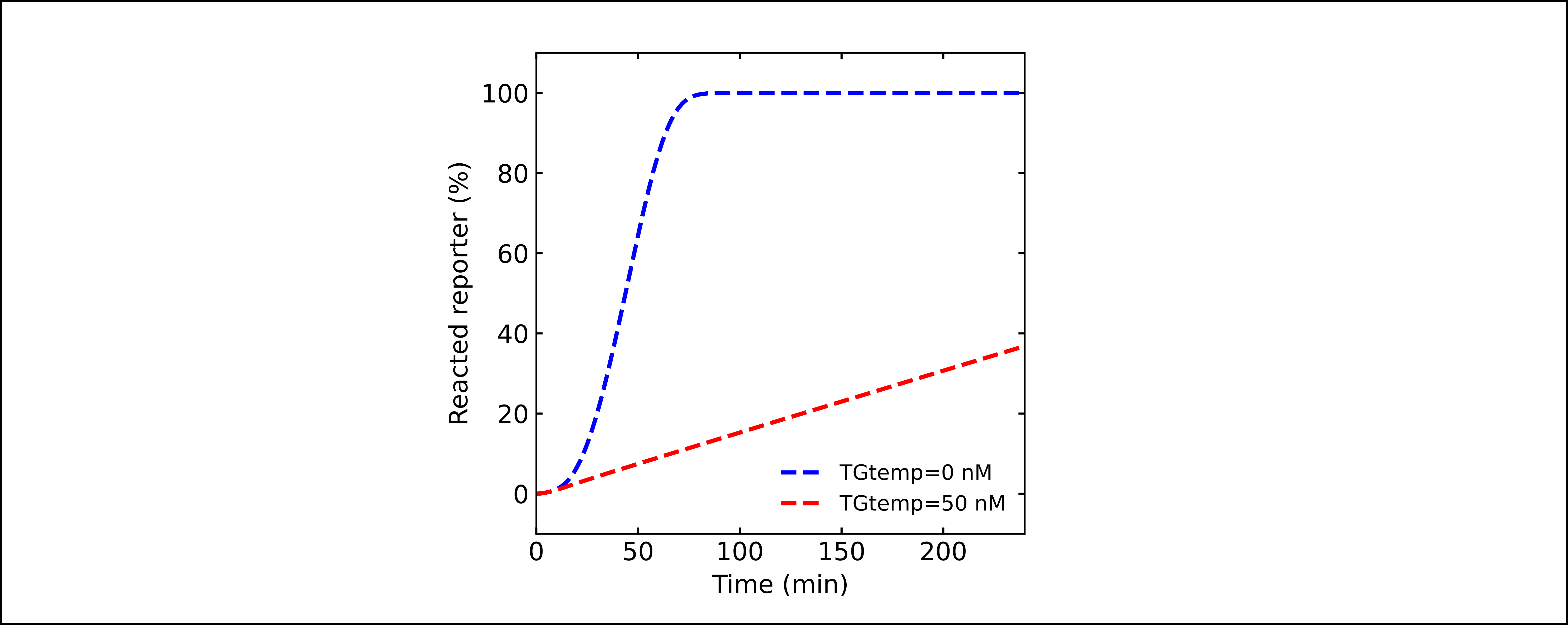
Threshold Simulation Results
Seesaw AND Element Simulations
A simulation of an AND gate using the seesaw gate design from Scaling Up Digital Circuit Computation with DNA Strand Displacement Cascades (Qian and Winfree *Science* 2011).
- Useful Features:
specifying threshold gates in molecular_species()
globally changing rate constants with global_rate_constants()
changing indiviudal rate constants within molecular_species()
changing initial conditions within molecular_species()
ctRSD seesaw element simulation
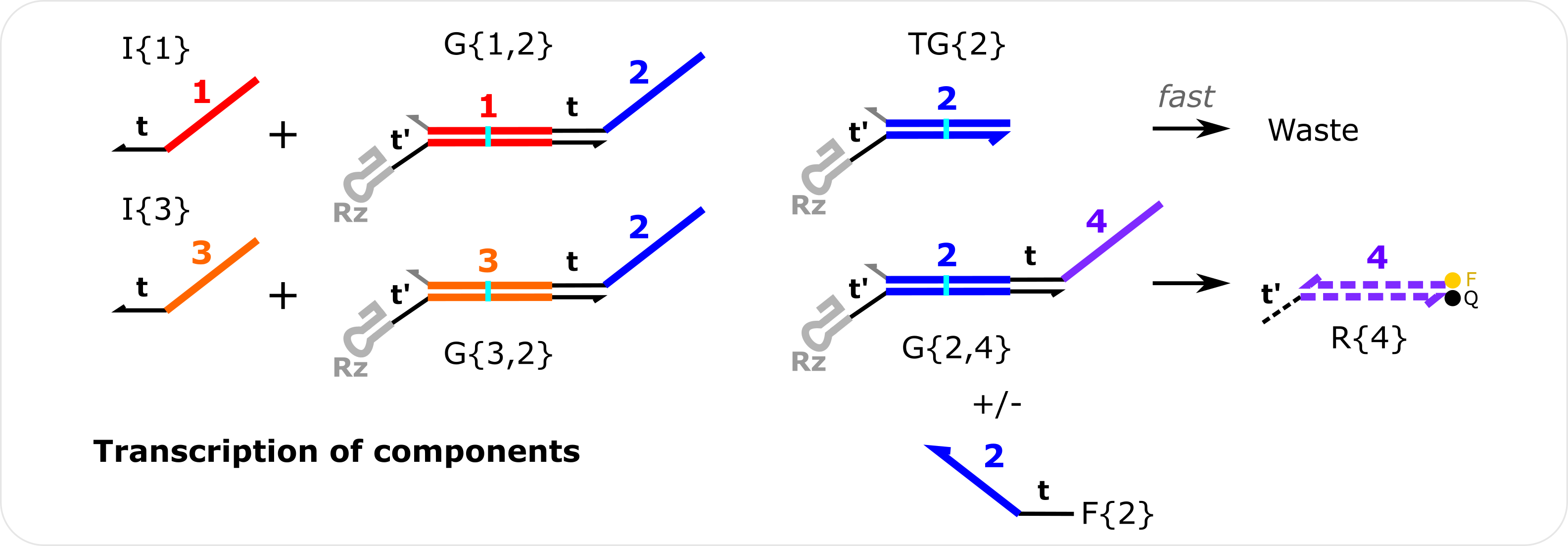
ctRSD Seesaw Simulation
ctRSD Seesaw Simulation Comparison Python Script can be found here
# auxiliary packages needed in the script below, e.g., plotting
import numpy as np
import matplotlib.pyplot as plt

# importing simulator
import sys
sys.path.insert(1,'filepath to simulator location on local computer')
import ctRSD_simulator_200 as RSDs # import latest version of the simulator


# create the model instance
model = RSDs.RSD_sim() # default # of domains (5 domains)

# specify species involved in the system
model.molecular_species('I{1}',DNA_con=25)
model.molecular_species('I{3}',DNA_con=25)

model.molecular_species('G{1,2}',DNA_con=16)
model.molecular_species('G{3,2}',DNA_con=16)

model.molecular_species('TG{2}',DNA_con=30)

model.molecular_species('G{2,4}',DNA_con=25)
model.molecular_species('F{2}',DNA_con=25)

model.molecular_species('R{4}',ic=500)

# simulating the model
t_sim = np.linspace(0,4,1001)*3600 # seconds
model.simulate(t_sim) # simulate the model

# pull out the species from the model solution to plot
S4 = model.output_concentration('S{4}')

# simple plotting code
plt.plot(t_sim,S4,color='purple')
plt.xlabel('Time (s)')
plt.ylabel('Concentration (nM)')
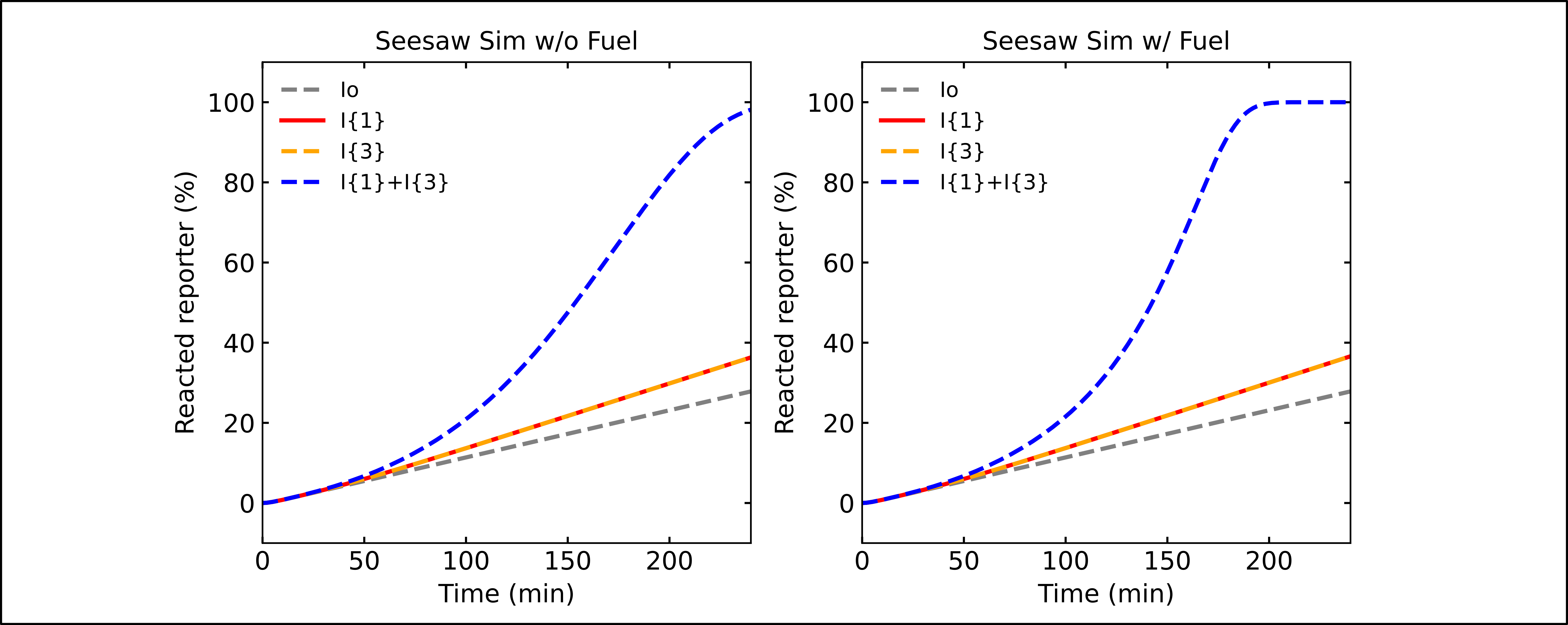
ctRSD Seesaw Simulation Results
DNA seesaw AND element simulation
This simulation mimics a DNA strand displacment reaction by setting DNA_con to 0 for all species and specifying only initial concentrations. Thus, only a fixed amount of each species is present and no transcription occurs.
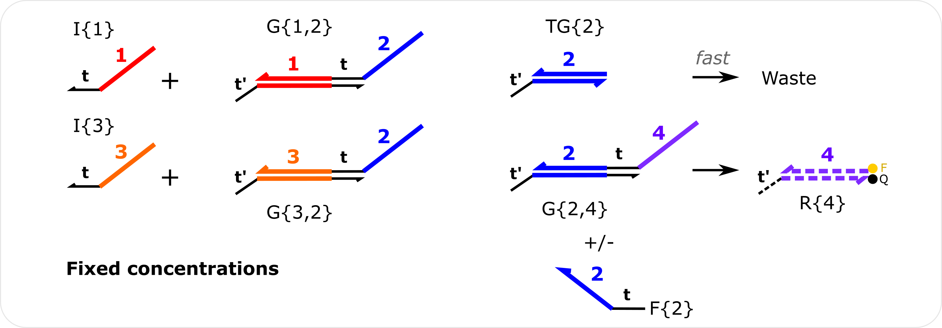
DNA Seesaw Simulation
DNA Seesaw Simulation Python Script can be found here
# auxiliary packages needed in the script below, e.g., plotting
import numpy as np
import matplotlib.pyplot as plt

# importing simulator
import sys
sys.path.insert(1,'filepath to simulator location on local computer')
import ctRSD_simulator_200 as RSDs # import latest version of the simulator


# create the model instance
model = RSDs.RSD_sim() # default # of domains (5 domains)

# changing rate constants to match those used in 2011 DNA computing paper
model.global_rate_constants(krev=5e4/1e9,krsd=5e4/1e9,krsdF=5e4/1e9,kth=2e6/1e9,krep=5e4/1e9)

# specify species involved in the system
# here only initial conditions are used so there is only a fixed concentration of each component added
model.molecular_species('I{1}',ic=90)
model.molecular_species('I{3}',ic=90)

model.molecular_species('G{1,2}',ic=100)
model.molecular_species('G{3,2}',ic=100)

model.molecular_species('TG{2}',ic=120)

model.molecular_species('G{2,4}',ic=200)
model.molecular_species('F{2}',ic=200)

model.molecular_species('R{4}',ic=150)

# simulating the model
t_sim = np.linspace(0,4,1001)*3600 # seconds
model.simulate(t_sim) # simulate the model

# pull out the species from the model solution to plot
S4 = model.output_concentration('S{4}')

# simple plotting code
plt.plot(t_sim,S4,color='purple')
plt.xlabel('Time (s)')
plt.ylabel('Concentration (nM)')
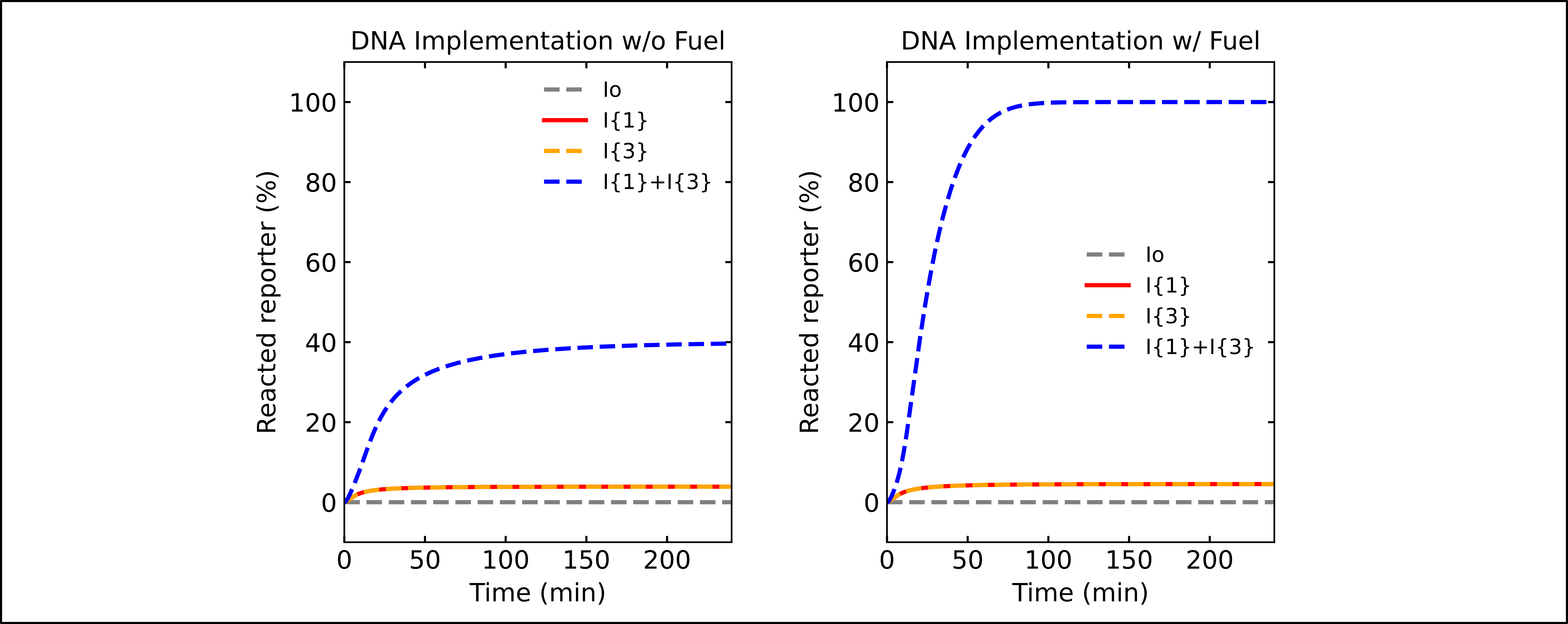
DNA Seesaw Simulation Results
Comparator Gate Simulation
Comparator Gate simulation shows a basic comparator gate reaction. This features shows the ability for a ctRSD circuit that compares the production rate of two inputs and only lets the input with the higher rate of product to the next layer of the circuit. Comparator gates are designed to function like the annihilator gates from Scaling Up Molecular Pattern Recognition with DNA-Based Winner-Take-All Neural Networks (Cherry and Qian *Nature* 2018).
- Useful Features:
specifying more than the default number of domains within RSD_sim()
specifying comparator gates in molecular_species()
globally changing rate constants with global_rate_constants()
changing indiviudal rate constants within molecular_species()
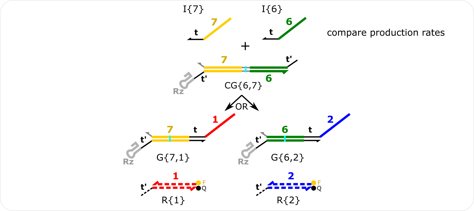
CG Simulation
CG Simulation Python Script can be found here
# auxiliary packages needed in the script below, e.g., plotting
import numpy as np
import matplotlib.pyplot as plt

# importing simulator
import sys
sys.path.insert(1,'filepath to simulator location on local computer')
import ctRSD_simulator_200 as RSDs # import latest version of the simulator


# create the model instance
model = RSDs.RSD_sim(7) # specifying the domains as the highest index in the simulated system below

# specify species involved in the system
model.molecular_species('I{6}',DNA_con=25)
model.molecular_species('I{7}',DNA_con=10)

model.molecular_species('CG{6,7}',DNA_con=45)

model.molecular_species('G{6,2}',DNA_con=15)
model.molecular_species('G{7,1}',DNA_con=15)

model.molecular_species('R{1}',ic=500)
model.molecular_species('R{2}',ic=500)

# simulating the model
t_sim = np.linspace(0,4,1001)*3600 # seconds
model.simulate(t_sim,smethod='BDF') # simulate the model ('BDF' method can speed up CG simulations)

# pull out the species from the model solution to plot
S1 = model.output_concentration('S{1}')
S2 = model.output_concentration('S{2}')

# simple plotting code
plt.plot(t_sim,S1,color='red')
plt.plot(t_sim,S2,color='blue')
plt.xlabel('Time (s)')
plt.ylabel('Concentration (nM)')
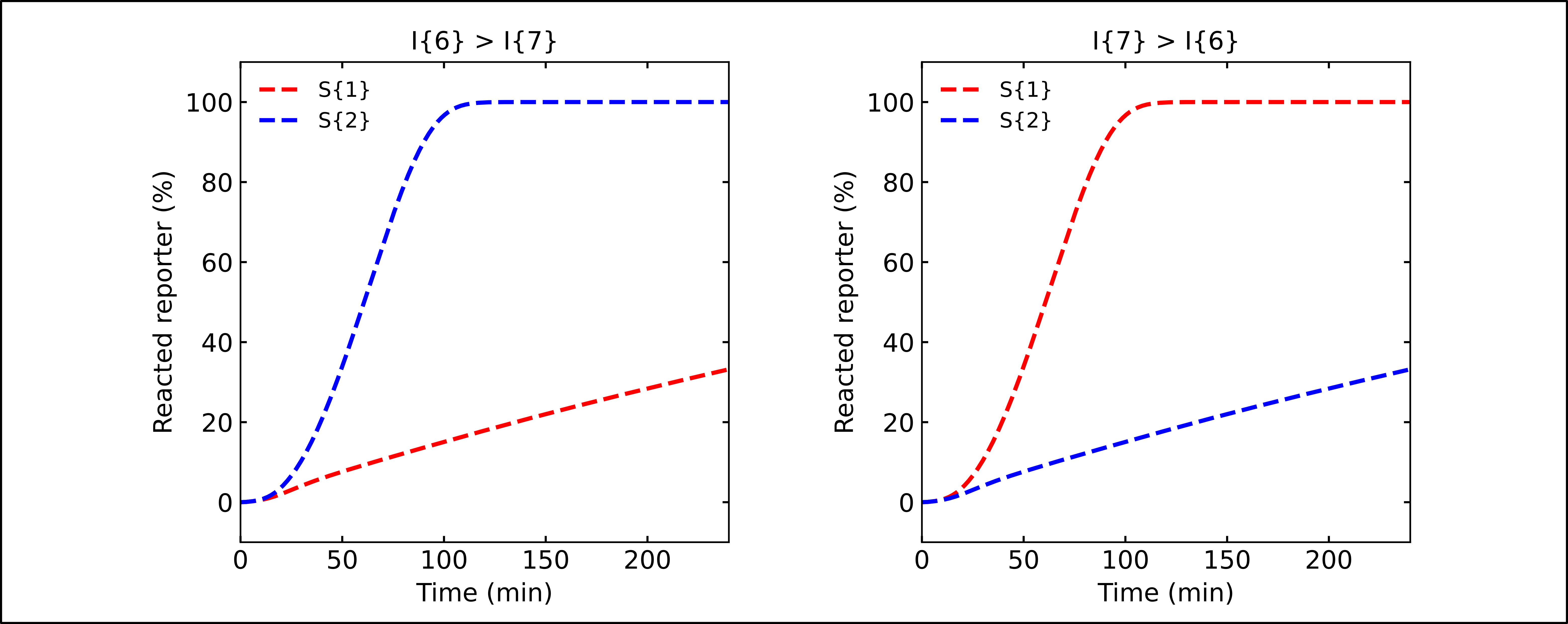
CG Simulation Results
The CG grid simulation is another example using a basic CG system that shows many more input template concentration combinations for the two inputs in the system.
CG Grid Simulation Python Script can be found here
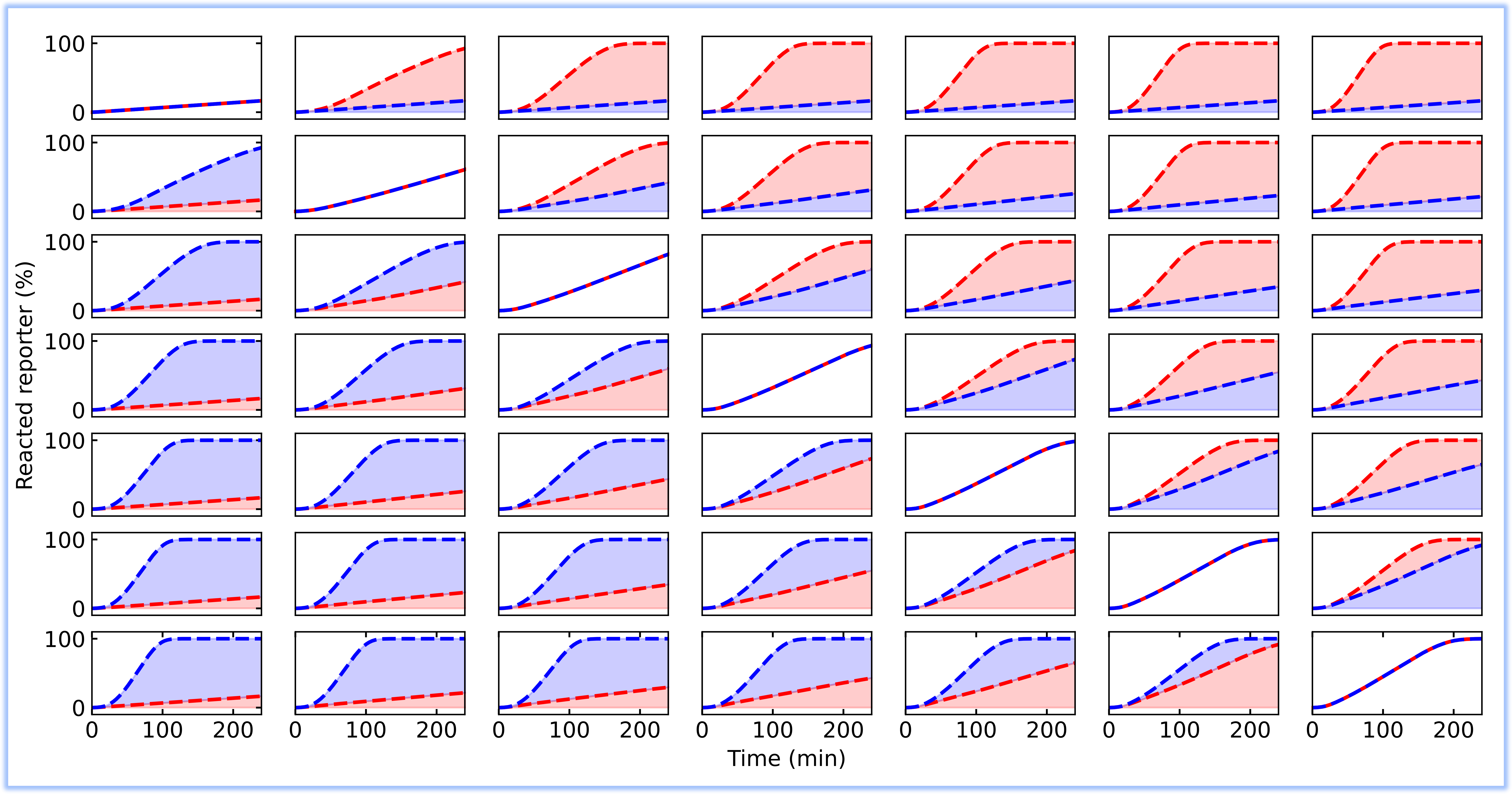
CG Grid Simulation Results
Three Comparator Gate Simulation
Three Comparator Gate Simulation is an extension of the comparator gate simulation that compares the rate of production of three inputs by using multiple comparator gates that encompass the pairwise comparisons of the inputs.
- Useful Features:
simulating relatively large circuits
specifying more than the default number of domains within RSD_sim()
specifying comparator gates in molecular_species()
globally changing rate constants with global_rate_constants()
changing indiviudal rate constants within molecular_species()
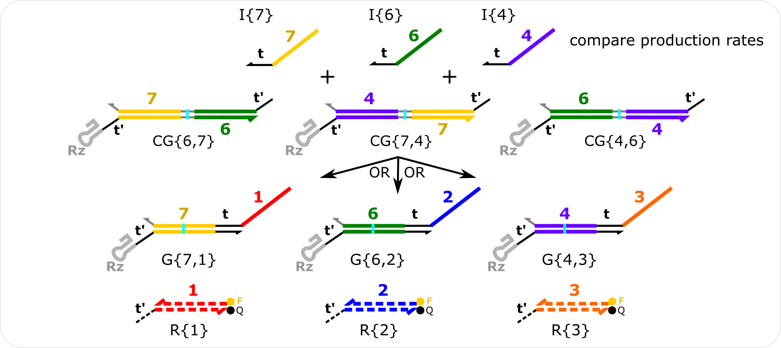
Three CG Simulation The model is set up such that the same input domain cannot be repeated in the same index for two gates. For example, CG{6,7} and CG{4,7} will result in an incorrect result because both gates have domain 7 in the second index. This should be changed to CG{6,7} and CG{7,4} so that domain 7 is in a different index for the two gates.
Three CG Simulation Python Script can be found here
# auxiliary packages needed in the script below, e.g., plotting
import numpy as np
import matplotlib.pyplot as plt

# importing simulator
import sys
sys.path.insert(1,'filepath to simulator location on local computer')
import ctRSD_simulator_200 as RSDs # import latest version of the simulator


# create the model instance
model = RSDs.RSD_sim(7) # specifying the domains as the highest index in the simulated system below

# increasing the forward strand displacement rate constant for all CG
model.global_rate_constants(krsdCG=5e5/1e9)

# specify species involved in the system
model.molecular_species('I{7}',DNA_con=50)
model.molecular_species('I{6}',DNA_con=30)
model.molecular_species('I{4}',DNA_con=20)

model.molecular_species('CG{6,7}',DNA_con=45)
model.molecular_species('CG{7,4}',DNA_con=45)
model.molecular_species('CG{4,6}',DNA_con=45)

model.molecular_species('G{6,2}',DNA_con=15)
model.molecular_species('G{7,1}',DNA_con=15)
model.molecular_species('G{4,3}',DNA_con=15)

model.molecular_species('R{1}',ic=500)
model.molecular_species('R{2}',ic=500)
model.molecular_species('R{3}',ic=500)

# simulating the model
t_sim = np.linspace(0,6,1001)*3600 # seconds
model.simulate(t_sim,smethod='BDF') # simulate the model ('BDF' method can speed up CG simulations)

# pull out the species from the model solution to plot
S1 = model.output_concentration('S{1}')
S2 = model.output_concentration('S{2}')
S3 = model.output_concentration('S{3}')

# simple plotting code
plt.plot(t_sim,S1,color='red')
plt.plot(t_sim,S2,color='blue')
plt.plot(t_sim,S3,color='orange')
plt.xlabel('Time (s)')
plt.ylabel('Concentration (nM)')
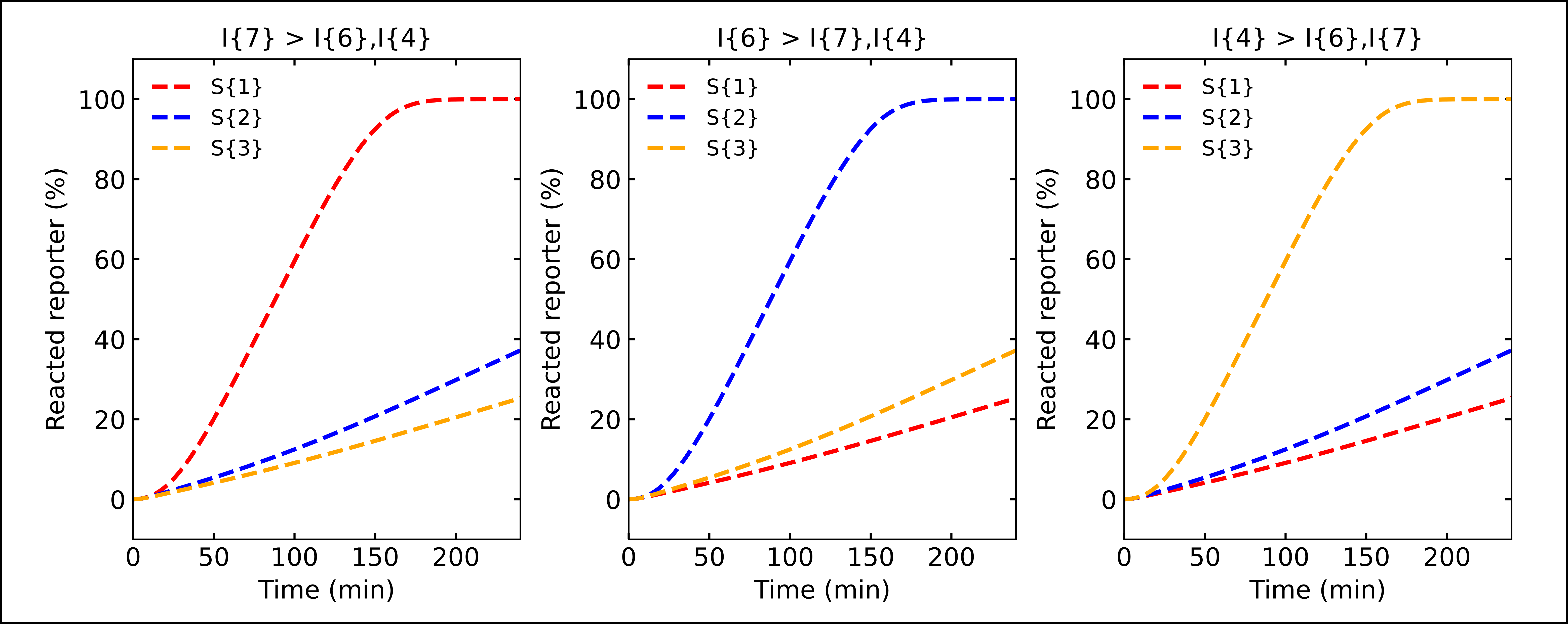
Three CG Simulation Results