Simple Examples
Individual scripts for the examples are shown below with links to the scripts on GitHub (the GitHub scripts have additional plotting features).
A Jupyter Notebook of these examples can be found here
Single ctRSD Gate Reaction
Simulating the system below
- Useful Features:
overveiw of setting up a basic simulation
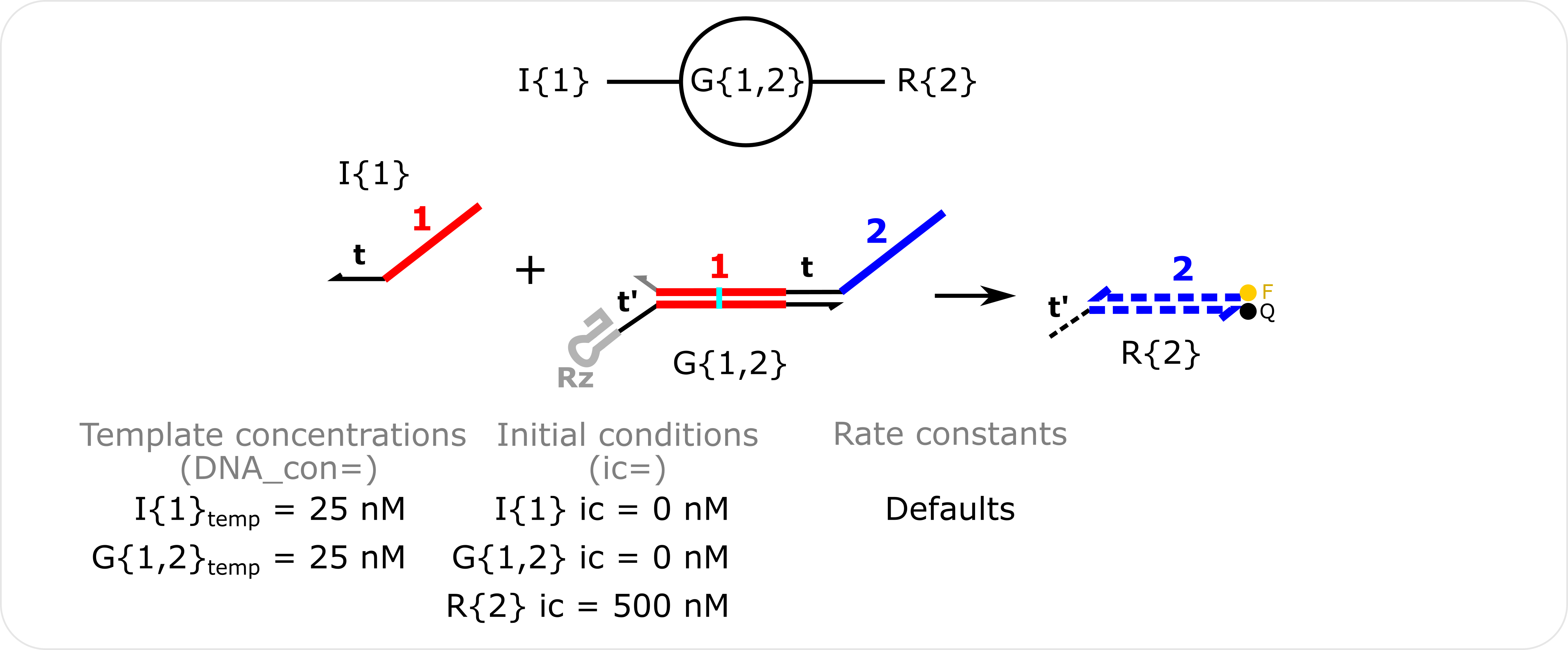
Single ctRSD Gate Reaction Template concentrations are specified with the DNA_con input in molecular_species() and non-zero initial conditions are specified with the ic input in molecular_species().
Single ctRSD Gate Reaction Python Script can be found here
# auxiliary packages needed in the script below, e.g., plotting
import numpy as np
import matplotlib.pyplot as plt

# importing simulator
import sys
sys.path.insert(1,'filepath to simulator location on local computer')
import ctRSD_simulator_200 as RSDs # import latest version of the simulator


# create the model instance
model = RSDs.RSD_sim() # default # of domains (5 domains)

# specify species involved in the system
model.molecular_species('I{1}',DNA_con=25)
model.molecular_species('G{1,2}',DNA_con=25)
model.molecular_species('R{2}',ic=500)

# simulating the model
t_sim = np.linspace(0,3,1001)*3600 # simulating from 0 to 3 hours with 1000 increments (*3600 converts to seconds)
model.simulate(t_sim) # simulate the model

# pull out the species from the model solution to plot
S2 = model.output_concentration('S{2}') # S{2} is the output of a reacted reporter (R{2})
I1 = model.output_concentration('I{1}') # concentration of I{1} as a function of time
G12 = model.output_concentration('G{1,2}') # concentration of G{1,2} as a function of time
# etc...

# simple plotting code
plt.plot(t_sim,S2)
plt.plot(t_sim,I1,color='red')
plt.plot(t_sim,G12,color='green')
plt.xlabel('Time (s)')
plt.ylabel('Concentration (nM)')
Two-Layer Cascade Simulation
Simulating the system below
- Useful Features:
overveiw of setting up a basic simulation
globally changing rate constants with global_rate_constants()
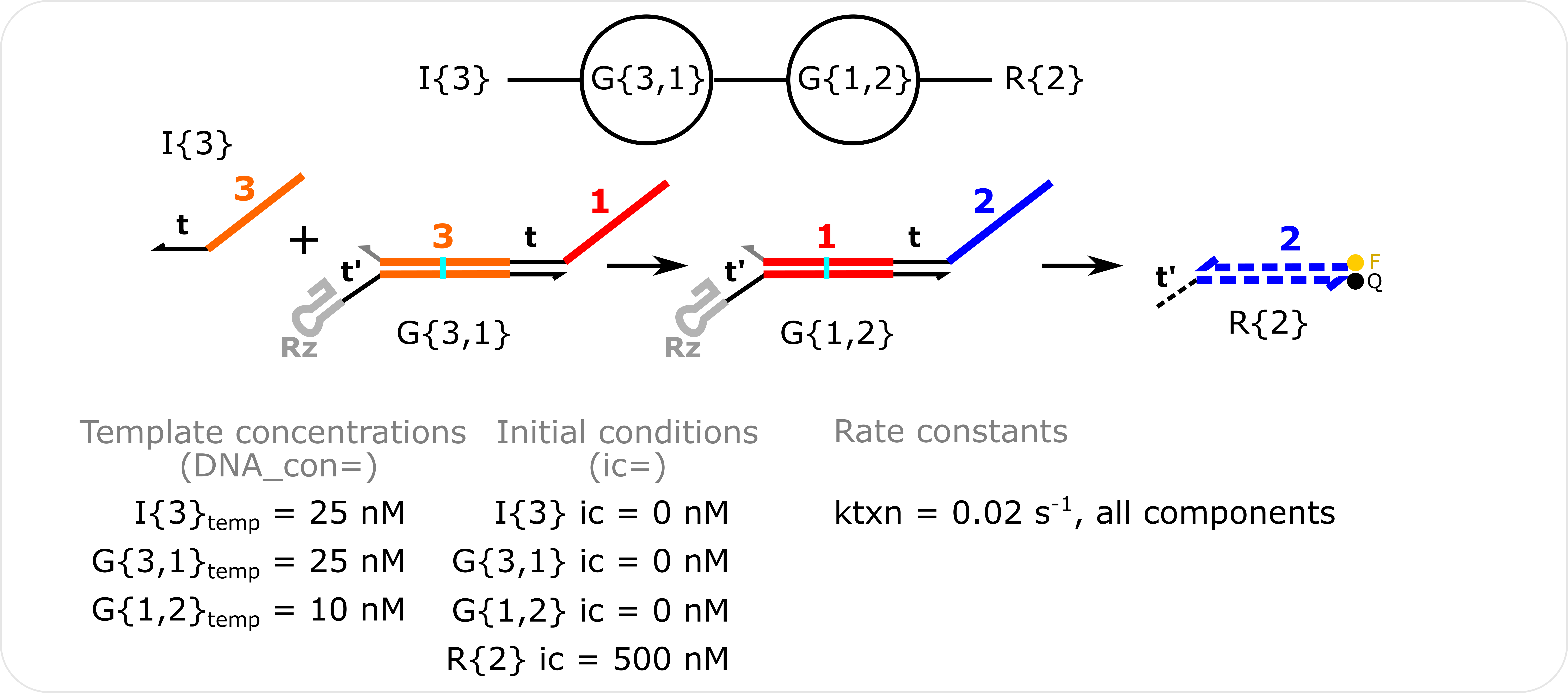
Two-Layer Cascade Simulation Template concentrations are specified with the DNA_con input in molecular_species() and non-zero initial conditions are specified with the ic input in molecular_species(). The transcription rate constant (ktxn) is changed for all species in global_rate_constants().
Two Layer Cascade Simulation Python Script can be found here
# auxiliary packages needed in the script below, e.g., plotting
import numpy as np
import matplotlib.pyplot as plt

# importing simulator
import sys
sys.path.insert(1,'filepath to simulator location on local computer')
import ctRSD_simulator_200 as RSDs # import latest version of the simulator


# create the model instance
model = RSDs.RSD_sim() # default # of domains (5 domains)

model.global_rate_constants(ktxn=0.02) # changing the global transcription rate constant

# specify species involved in the system
model.molecular_species('I{3}',DNA_con=25)
model.molecular_species('G{3,1}',DNA_con=25)
model.molecular_species('G{1,2}',DNA_con=10)
model.molecular_species('R{2}',ic=500)

# simulating the model
t_sim = np.linspace(0,3,1001)*3600 # simulating from 0 to 3 hours with 1000 increments (*3600 converts to seconds)
model.simulate(t_sim) # simulate the model

# pull out the species from the model solution to plot
S2 = model.output_concentration('S{2}') # S{2} is the output of a reacted reporter (R{2})
I3 = model.output_concentration('I{3}') # concentration of I{3} as a function of time
G12 = model.output_concentration('G{1,2}') # concentration of G{1,2} as a function of time
# etc...

# simple plotting code
plt.plot(t_sim,S2)
plt.plot(t_sim,I3,color='red')
plt.plot(t_sim,G12,color='green')
plt.xlabel('Time (s)')
plt.ylabel('Concentration (nM)')
Fan-Out Simulation
Simulating the system below
- Useful Features:
overveiw of setting up a basic simulation
globally changing rate constants with global_rate_constants()
changing indiviudal rate constants within molecular_species()
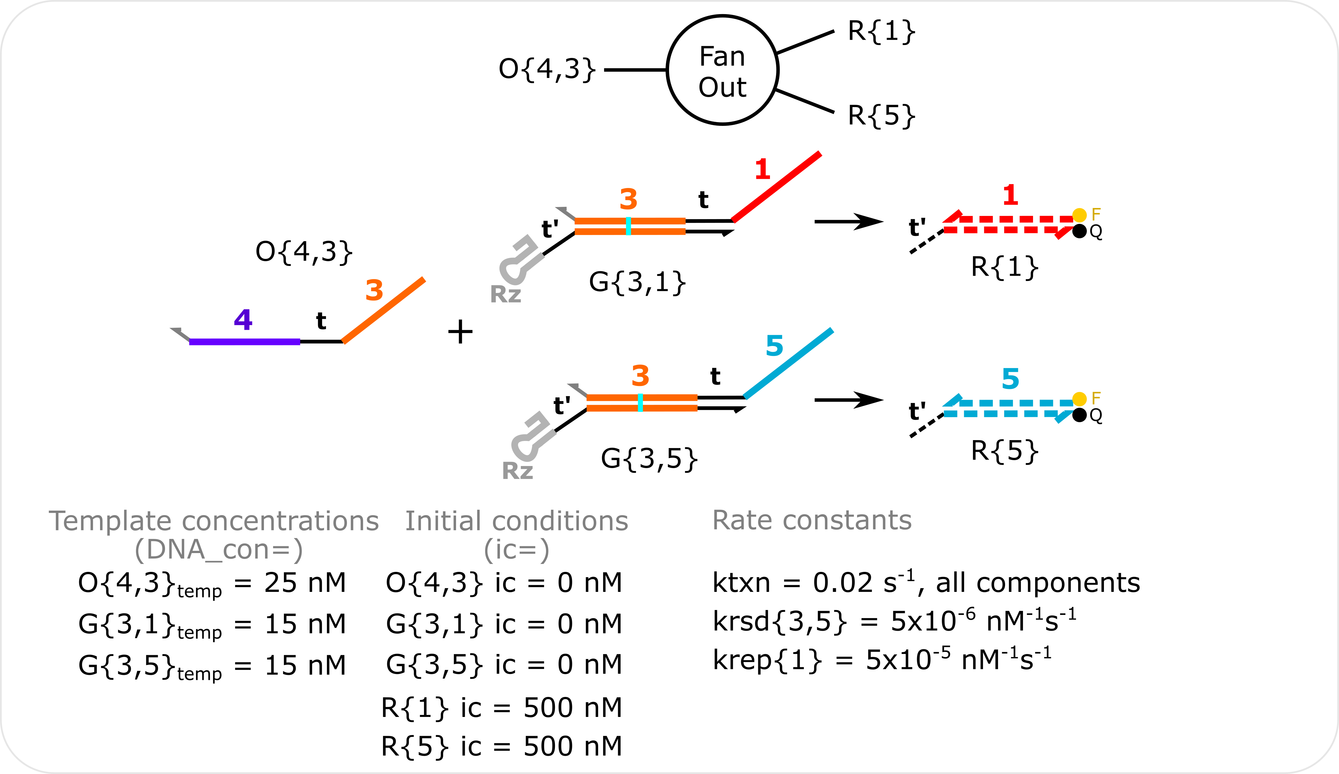
Fan-Out Simulation Template concentrations are specified with the DNA_con input in molecular_species() and non-zero initial conditions are specified with the ic input in molecular_species(). The transcription rate constant (ktxn) is changed for all species in global_rate_constants(). krsd{3,5} is changed in molecular_species() when G{3,5} is specified. krep{1} is changed in *molecular_species() when R{1} is specified.
Fan Out Simulation Python Script can be found here
# auxiliary packages needed in the script below, e.g., plotting
import numpy as np
import matplotlib.pyplot as plt

# importing the simulator
import sys
sys.path.insert(1,'filepath to simulator location on local computer')
import ctRSD_simulator_200 as RSDs # import latest version of the simulator


# create the model instance
model = RSDs.RSD_sim() # default # of domains (5 domains)

model.global_rate_constants(ktxn=0.02) # changing the global transcription rate constant

# specify species involved in the system
model.molecular_species('O{4,3}',DNA_con=25)
model.molecular_species('G{3,1}',DNA_con=15)
model.molecular_species('G{3,5}',DNA_con=15,krsd=5e-6) # changing krsd{3,5}
model.molecular_species('R{1}',ic=500,krep=5e-5) # changing krep{1}
model.molecular_species('R{5}',ic=500)

# simulating the model
t_sim = np.linspace(0,3,1001)*3600 # simulating from 0 to 3 hours with 1000 increments (*3600 converts to seconds)
model.simulate(t_sim) # simulate the model

# pull out the species from the model solution to plot
S1 = model.output_concentration('S{1}') # S{1} is the output of reacted reporter R{1}
S5 = model.output_concentration('S{5}') # S{5} is the output of reacted reporter R{5}
# etc...

# simple plotting code
plt.plot(t_sim,S1,color='red')
plt.plot(t_sim,S5,color='cyan')
plt.xlabel('Time (s)')
plt.ylabel('Concentration (nM)')
Fan-Out Fan-In Simulation
Simulating the system below
- Useful Features:
overveiw of setting up a basic simulation
specifying more than the default number of domains within RSD_sim()
globally changing rate constants with global_rate_constants()
changing indiviudal rate constants within molecular_species()
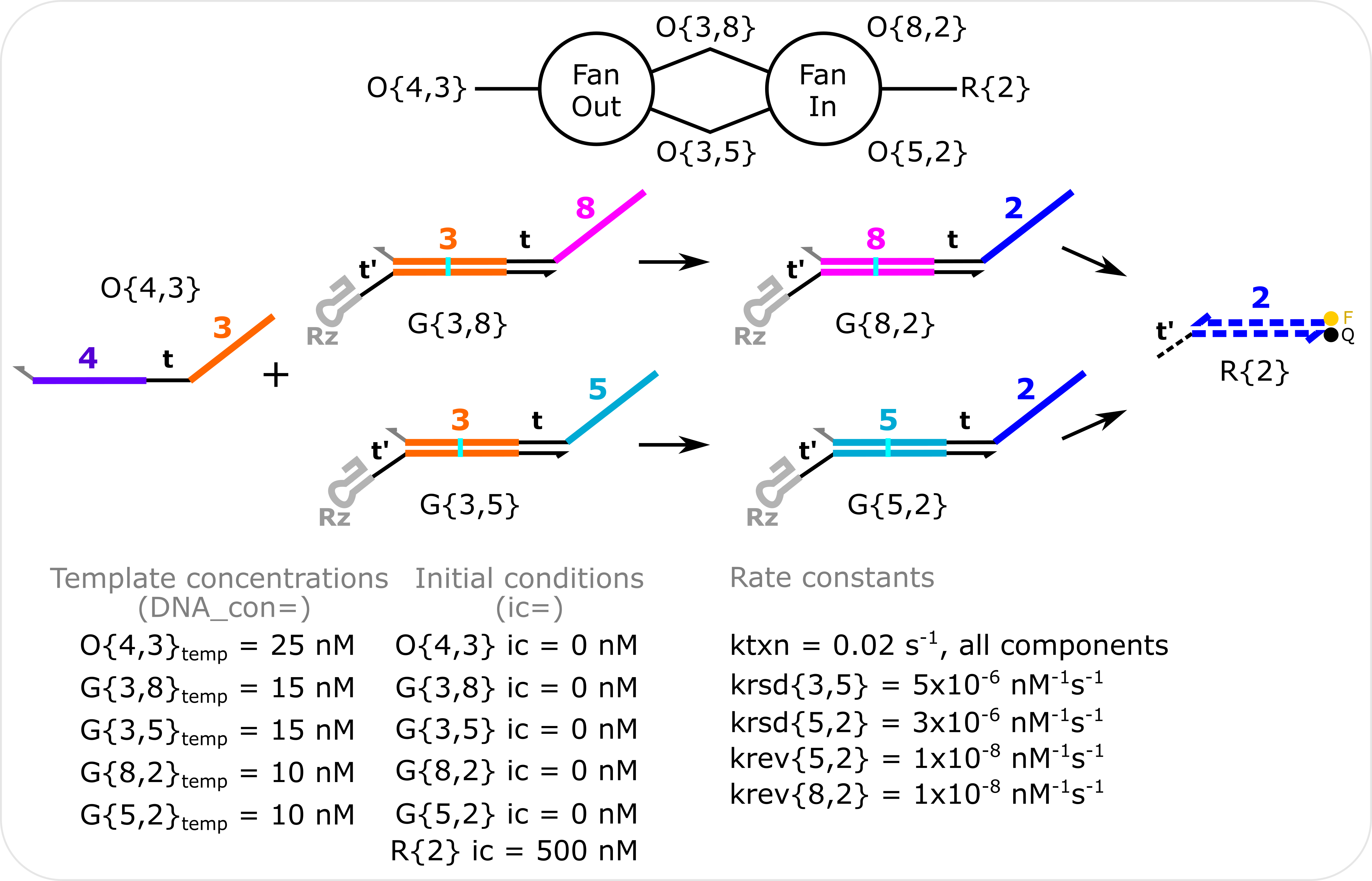
Fan-Out Fan-In Simulation Template concentrations are specified with the DNA_con input in molecular_species() and non-zero initial conditions are specified with the ic input in molecular_species(). The transcription rate constant (ktxn) is changed for all species in global_rate_constants(). Rate constants for individual species are changed in molecular_species(). The total domains initialized in the model is increased to 8 when the model is initialized in RSD_sim().
Fan Out Fan In Simulation Python Script can be found here
# auxiliary packages needed in the script below, e.g., plotting
import numpy as np
import matplotlib.pyplot as plt

# importing simulator
import sys
sys.path.insert(1,'filepath to simulator location on local computer')
import ctRSD_simulator_200 as RSDs # import latest version of the simulator


# create the model instance
model = RSDs.RSD_sim(8) # increasing # of domains to match highest index in the system

model.global_rate_constants(ktxn=0.02) # changing the global transcription rate constant

# specify species involved in the system
model.molecular_species('O{4,3}',DNA_con=25)
model.molecular_species('G{3,8}',DNA_con=15)
model.molecular_species('G{3,5}',DNA_con=15,krsd=5e-6) # changing krsd{3,5}
model.molecular_species('G{8,2}',DNA_con=10,krev=1e-8) # changing krev{8,2}
model.molecular_species('G{5,2}',DNA_con=10,krsd=3e-6,krev=1e-8) # changing krsd{5,2} and krev{5,2}
model.molecular_species('R{2}',ic=500)

# simulating the model
t_sim = np.linspace(0,3,1001)*3600 # simulating from 0 to 3 hours with 1000 increments (*3600 converts to seconds)
model.simulate(t_sim) # simulate the model

# pull out the species from the model solution to plot
S2 = model.output_concentration('S{2}')  # S{2} is the output of a reacted reporter (R{2})
# etc...

# simple plotting code
plt.plot(t_sim,S2,color='blue')
plt.xlabel('Time (s)')
plt.ylabel('Concentration (nM)')
Experimental Nomenclature
Simulating the systems below
- Useful Features:
overveiw of setting up a basic simulation
using expanded experimental nomenclature when specifying components within molecular_species()
globally changing rate constants with global_rate_constants()
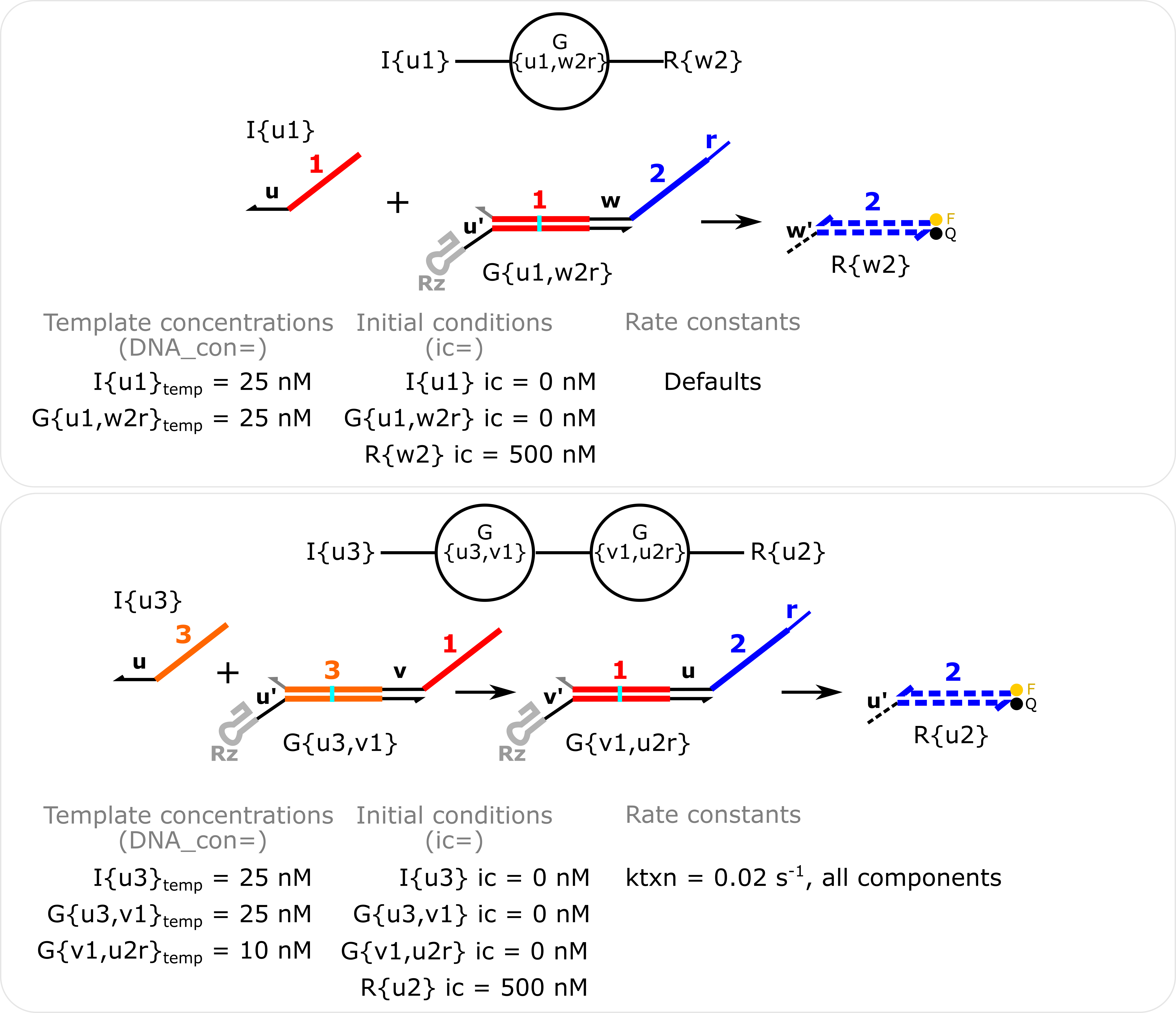
Single gate reaction and two layer cascade with experimental nomenclature In ctRSD circuit experiments different input and output toeholds are often used. This, and the inclusion of other additional domains, leads to an expanded nomenclature compared to what is used in the simulator. Experimentalists may want to use the expanded nomenclature in their simulations to keep track of how circuits are linked together. The simulator allows for this expanded nomenclature by ignoring any letters before or after the input-output indices of a component. The code below highlights this feature.
Note using the expanded nomenclature below does not change anything about the simulation. The simulator ignores the letters before or after the indices. This is merely a way to keep track of the experimental components in a simulation. If the different toeholds have different rate constants, these can be changed when each component is defined in molecular_species(), see Two toehold cascade simulation
Single ctRSD Gate Reaction with Experimental Nomenclature Python Script can be found here
# auxiliary packages needed in the script below, e.g., plotting
import numpy as np
import matplotlib.pyplot as plt

# importing simulator
import sys
sys.path.insert(1,'filepath to simulator location on local computer')
import ctRSD_simulator_200 as RSDs # import latest version of the simulator


# create the model instance
model = RSDs.RSD_sim() # default # of domains (5 domains)

# specify species involved in the system
model.molecular_species('I{u1}',DNA_con=25)
model.molecular_species('G{u1,w2r}',DNA_con=25)
model.molecular_species('R{w2}',ic=500)

# simulating the model
t_sim = np.linspace(0,3,1001)*3600 # simulating from 0 to 3 hours with 1000 increments (*3600 converts to seconds)
model.simulate(t_sim) # simulate the model

# pull out the species from the model solution to plot
S2 = model.output_concentration('S{w2}')  # S{w2} is the output of a reacted reporter (R{w2})
# etc...

# simple plotting code
plt.plot(t_sim,S2,color='blue')
plt.xlabel('Time (s)')
plt.ylabel('Concentration (nM)')
Two Layer Simulation with Experimental Nomenclature Python Script can be found here
# auxiliary packages needed in the script below, e.g., plotting
import numpy as np
import matplotlib.pyplot as plt

# importing simulator
import sys
sys.path.insert(1,'filepath to simulator location on local computer')
import ctRSD_simulator_200 as RSDs # import latest version of the simulator


# create the model instance
model = RSDs.RSD_sim() # default # of domains (5 domains)

model.global_rate_constants(ktxn=0.02) # changing the global transcription rate constant

# specify species involved in the system
model.molecular_species('I{u3}',DNA_con=25)
model.molecular_species('G{u3,v1}',DNA_con=25)
model.molecular_species('G{v1,u2r}',DNA_con=10)
model.molecular_species('R{u2}',ic=500)

# simulating the model
t_sim = np.linspace(0,3,1001)*3600 # simulating from 0 to 3 hours with 1000 increments (*3600 converts to seconds)
model.simulate(t_sim) # simulate the model

# pull out the species from the model solution to plot
S2 = model.output_concentration('S{u2}')
# etc...

# simple plotting code
plt.plot(t_sim,S2,color='blue')
plt.xlabel('Time (s)')
plt.ylabel('Concentration (nM)')